The beauty of math’s incompleteness or how self-references can beautifully screw things up
Table of Contents
“Logic is the hygiene that the mathematician practises to keep his ideas healthy and strong.”
— Hermann Weyl
I have a very special place for mathematics in my mind and heart.
Mathematics is above any other science. This is because the knowledge we gather in all other sciences are never absolutely true. All other sciences are based on observations and experiments, and eventually evidence accrues to a threshold that we can morally declare that something is true. Yet, it is not mathematically true, in other words, for any given pile of evidence about a given hypothesis $H$, we have $P(H) < 1$. In a pure philosophical sense, we can never be absolutely sure about scientific hypotheses. There will always be a certain degree of uncertainty even if we have a lot of evidence in favor of a given hypothesis. For mathematical theorems, which is the meat of mathematics, once they are proven, they are absolutely true, i.e. $P(H) = 1$. For example, imagine a galaxy very far away, and a million years from now, given the 5 axioms of Euclidian geometry, the theorem that the sum of the angles of a triangle is 180 degrees will still be true. It will always be true (given the 5 axioms of course).
That is how mathematics won my mind. Now, how it won my heart is a different story. It has to do with the beauty of math’s incompleteness, inconsistency, and undecidability. Which all stems from self-referential paradoxes.
Cantor and multiple infinities
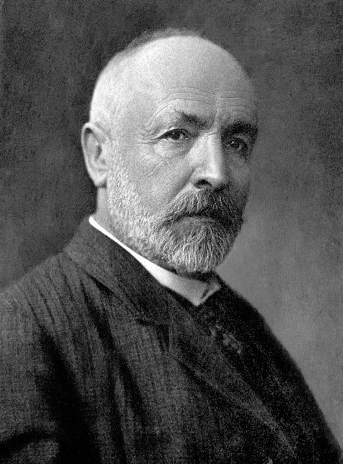
Let’s go back to 1874, when Georg Cantor proved that there are multiple infinities. Yes, that sounds crazy, but it is true.
Cantor is the father of set theory. Before him, the concept of a set was just a collection of objects and they were all finite collections. This dates back to Aristotle, and no one imagined that there was interesting things to say about sets. In order to put set theory on a solid footing, Cantor had to define what a set is. For finite sets, this was kinda trivial. However, for infinite sets, this is where things started to get interesting.
Cantor started exploring the properties of infinite sets. First, he analyzed the properties of the set of natural numbers $\mathbb{N}$. He then realized that the set of natural numbers is the same size as the set of the integers $\mathbb{Z}$ and the set of the rational numbers $\mathbb{Q}$. To show this, he had to come up with a way to compare the sizes of sets. He did this by defining a bijection between the set of natural numbers and the set of integers. A bijection is a function that is one-to-one and onto. In other words, it is a function that maps each element of the first set to a unique element of the second set, and each element of the second set to a unique element of the first set.
For example, the function
$$ f(n) = \begin{cases} -\frac{n}{2} & \text{if } n \text{ is even} \\ \frac{n+1}{2} & \text{if } n \text{ is odd} \end{cases} $$
is a bijection between the set of natural numbers and the set of integers.
It creates a one-to-one correspondence between the set of natural numbers and the set of integers:
| $f(n)$ | $\mathbb{N}$ | $\mathbb{Z}$ |
|---|---|---|
| f(0) | 0 | 0 |
| f(1) | 1 | 1 |
| f(2) | 2 | -1 |
| f(3) | 3 | 2 |
| f(4) | 4 | -2 |
| f(5) | 5 | 3 |
| f(6) | 6 | -3 |
Ok that was easy, we just proved that the set of natural numbers and the set of integers have the same size. Now let’s try to prove the same for the set of rational numbers $\mathbb{Q}$. The idea again is to find a bijection between the set of natural numbers and the set of rational numbers. We can represent the set of rational numbers as a grid of fractions:
$$ \begin{array}{cccc} \frac{1}{1} & \quad \frac{1}{2} & \quad \frac{1}{3} & \quad \cdots \\\\ \frac{2}{1} & \quad \frac{2}{2} & \quad \frac{2}{3} & \quad \cdots \\\\ \frac{3}{1} & \quad \frac{3}{2} & \quad \frac{3}{3} & \quad \cdots \\\\ \vdots & \quad \vdots & \quad \vdots & \quad \ddots \\\\ \end{array} $$
Now, we can’t just go row by row or column by column — that would never finish the first row! Instead, Cantor had a brilliant idea: traverse the grid diagonally in a zigzag pattern1.
$$ \begin{array}{ccccc} \frac{1}{1} & \rightarrow & \frac{1}{2} & \quad & \frac{1}{3} & \rightarrow & \frac{1}{4} & \cdots \\ & \swarrow & & \nearrow & & \swarrow & \\ \frac{2}{1} & & \frac{2}{2} & & \frac{2}{3} & & \frac{2}{4} & \cdots \\ \downarrow & \nearrow & & \swarrow & & & \\ \frac{3}{1} & & \frac{3}{2} & & \frac{3}{3} & & \frac{3}{4} & \cdots \\ & \swarrow & & \nearrow & & & \\ \frac{4}{1} & & \frac{4}{2} & & \frac{4}{3} & & \frac{4}{4} & \cdots \\ \vdots & & \vdots & & \vdots & & \vdots & \ddots \\ \end{array} $$
This gives us the sequence: $$ \frac{1}{1}, \frac{1}{2}, \frac{2}{1}, \frac{3}{1}, \frac{2}{2}, \frac{1}{3}, \frac{1}{4}, \frac{2}{3}, \frac{3}{2}, \frac{4}{1}, \ldots $$
But wait! We have a problem — many fractions represent the same rational number:
- $\frac{2}{2} = \frac{1}{1} = 1$
- $\frac{2}{4} = \frac{1}{2} = 0.5$
To create a true bijection, we need to skip these duplicates. We only keep fractions in lowest terms, where $\text{gcd}(\text{numerator}, \text{denominator}) = 1$.
After removing duplicates: $$\frac{1}{1}, \frac{1}{2}, \frac{2}{1}, \frac{3}{1}, \frac{1}{3}, \frac{1}{4}, \frac{2}{3}, \frac{3}{2}, \frac{4}{1}, \ldots$$
Ok we’re almost there. This is truly a bijection. However, it is a bijection between $\mathbb{N}$ and the set of positive rationals, $\mathbb{Q}^+$. To include all of $\mathbb{Q}$, we interleave positive and negative rationals (and zero). I won’t give the precise mathematical formula here because it is a bit messy, however here’s an algorithm describing the bijection:
- Start with $n$
- If $n = 0$, return $0$
- Otherwise:
- Let $k = \frac{n+1}{2}$ if $n$ is odd, $k = \frac{n}{2}$ if $n$ is even
- Find the $k$-th positive rational in our enumeration, call it $r$
- If $n$ is odd, return $r$
- If $n$ is even, return $-r$
This gives us the following bijection:
| $g(n)$ | $\mathbb{N}$ | $\mathbb{Q}^+$ enumeration | $\mathbb{Q}$ |
|---|---|---|---|
| g(0) | 0 | - | 0 |
| g(1) | 1 | 1st positive: $\frac{1}{1}$ | 1 |
| g(2) | 2 | 1st positive: $\frac{1}{1}$ | -1 |
| g(3) | 3 | 2nd positive: $\frac{1}{2}$ | $\frac{1}{2}$ |
| g(4) | 4 | 2nd positive: $\frac{1}{2}$ | $-\frac{1}{2}$ |
| g(5) | 5 | 3rd positive: $\frac{2}{1}$ | 2 |
| g(6) | 6 | 3rd positive: $\frac{2}{1}$ | -2 |
Q.E.D.! We have a bijection between $\mathbb{N}$ and $\mathbb{Q}$.
I went over all of these details because this diagonalization argument is a very important insight. Any set that can be put in a one-to-one correspondence with the set of natural numbers is called countable. Cantor showed that the set of rational numbers is countable.
Let’s see what happens when we try to apply the same argument to the set of real numbers $\mathbb{R}$. For the sake of simplicity, let’s consider the set of real numbers between 0 and 1, $\mathbb{R}_{(0,1)}$.
Let’s assume that we have a bijection $f$ between $\mathbb{N}$ and $\mathbb{R}_{(0,1)}$. This would give us the following table:
| $f(n)$ | $\mathbb{N}$ | $\mathbb{R}_{(0,1)}$ |
|---|---|---|
| f(0) | 0 | 0.011… |
| f(1) | 1 | 0.111… |
| f(2) | 2 | 0.112… |
| … | … | … |
Note that the real number $f(n)$ is the $n$-th real number in the list.
Now, let’s construct a new real number $x$ that is not in the list. We will do this by constructing a real number that is different from the $n$-th real number in the list for all $n$. We just add 1 to the $n$-th digit of the $n$-th real number in the list. For example, for the first real number in the list, we add 1 to the first digit, for the second real number in the list, we add 1 to the second digit, and so on.
This gives us the following real number: $0.123\ldots$ By construction, this real number is not in the list, since it differs from the first real number in the list by 1 in the first digit, from the second real number in the list by 1 in the second digit, and so on.
This is a contradiction, since we assumed that $f$ was a bijection.
Now, this is where self-reference strikes first in this post, and probably in the history of mathematics. When we construct the diagonal number $x$, we’re creating something that:
- Refers to the entire supposed list of real numbers.
- Defines itself in opposition to that list — “I differ from the 1st number at position 1, from the 2nd at position 2…”.
- Uses the list to prove the list is incomplete.
Ultimately, this is where Cantor found the first example of a set that is not countable. There’s no way to pair the set of natural numbers with the set of real numbers between 0 and 1. Therefore, the set of real numbers between 0 and 1 is not countable. This is called the Cantor’s diagonal argument.
This is a very important insight. It shows that there are different sizes of infinity. Yes, that is mind-blowing and paradoxically beautiful.
Cantor called the size of the set of natural numbers $\aleph_0$, and conjectured that the set of real numbers is $\aleph_1$. This is called the continuum hypothesis (CH).
Russell and the barber paradox
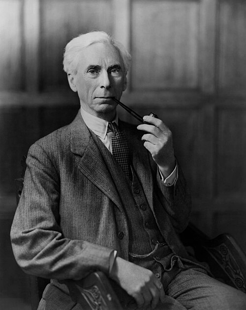
Now let’s fast forward to 1901. Set theory was still in its infancy, yet it was starting to be accepted by the mathematical community. This is where Bertrand Russell after attending the first World Congress of Philosophy in Paris in 1900, was impressed by the work of Peano who was using set theory to formalize mathematics.
He embarked on a journey to formalize mathematics using set theory. However, he stumbled upon a paradox. Set theory is very lenient with the definition of sets. For example, we can define the set of all sets that are not members of themselves:
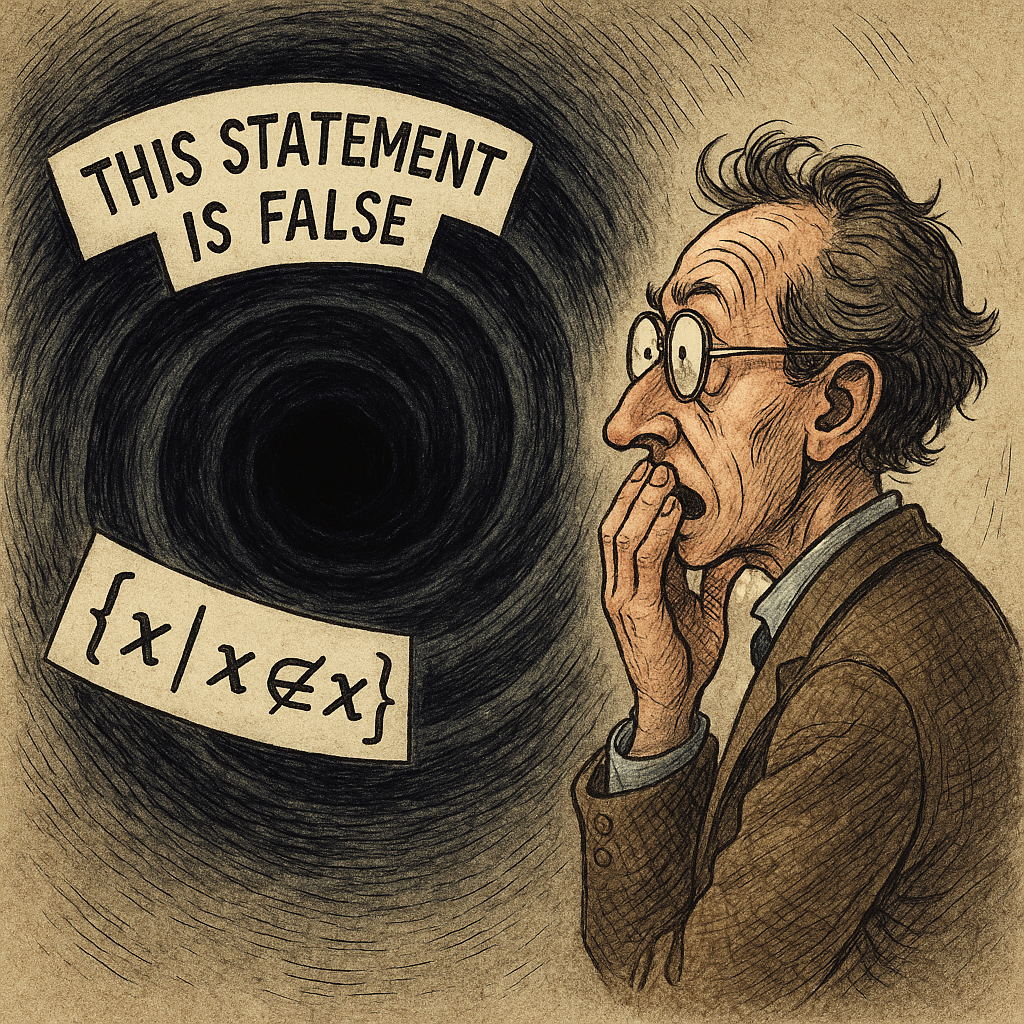
$$ R = \{ x \mid x \notin x \} $$
Now what happens if we ask the question: is $R$ a member of itself? If $R$ is a member of itself, then it is not a member of itself. If $R$ is not a member of itself, then it is a member of itself.
To put more simply, Russell gave the simple analogy: imagine a barber who shaves all men who do not shave themselves. Now, the question is: does the barber shave himself? If he does, then he does not shave himself. If he does not shave himself, then he does shave himself.
I can even given an even more simple example: the statement “this statement is false” is a paradox. If it is true, then it is false. If it is false, then it is true.
Or suppose that I go out and shout out loud: “I am lying”. If I am lying, then I am not lying. If I am not lying, then I am lying.
All of these examples boil down to the same thing: we cannot have a set of all sets that are not members of themselves.
This is called the Russell’s paradox. And yet again, we have self-reference creating a paradox. Personally, I find Cantor’s multiple infinities more beautiful than Russell’s paradox. But I acknowledge that Russell’s paradox is way simpler and more accessible to the general public.
Gödel and the incompleteness theorem
Fasten your seatbelts, this is going to be a wild ride. But first, a little bit of history.
In 1900, during the second International Congress of Mathematicians in Paris, David Hilbert, arguably the most important mathematician of the 20th century, gave a list of 23 problems that he thought would be the most important to solve in the century. These became known as the Hilbert’s problems. Right there in the second problem, Hilbert posed the following problem:
The compatibility of the arithmetical axioms.
Later, Hilbert recasted his “Second Problem” at the eighth International Congress of Mathematicians in Bologna. He posed three questions:
- Was mathematics complete?
- Was mathematics consistent?
- Was mathematics decidable?
Hilbert believed that mathematics could be put on a completely secure foundation by answering these questions. Gödel would shatter the dream of a complete and consistent mathematics. And later, Turing would show that mathematics is not decidable.
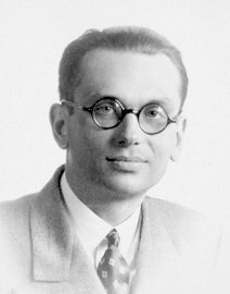
Gödel’s incompleteness theorems2 are composed of two theorems. Let’s start with the first incompleteness theorem, which Gödel proved in 1931 in front of an audience that comprised of no one other than Von Neumann, who allegedly was so impressed by Gödel’s work that he remarked:
It’s all over.
The first incompleteness theorem
The First Incompleteness Theorem states:
For any consistent formal system $F$ that is powerful enough to express basic arithmetic3, there exists a statement $G$ in the language of $F$ such that:
- $G$ is true (when interpreted as a statement about natural numbers)
- $G$ cannot be proven within $F$
- $\neg G$ (not $G$) cannot be proven within $F$ either
In other words: truth and provability are not the same thing!
Gödel’s genius was realizing he could make mathematical statements talk about mathematical statements.
Step 1: Gödel numbering — the encoding trick
Gödel assigned a unique natural number to every mathematical symbol, expression, and proof. Think of it like ASCII encoding for math:
Basic symbols get prime numbers:
0→ 2=→ 3+→ 5(→ 7)→ 11- etc.
Gödel used a system based on prime factorization. He first assigned a unique natural number to each basic symbol in the formal language of arithmetic with which he was dealing.
To encode an entire formula, which is a sequence of symbols, Gödel used the following system. Given a sequence $(x_{1},x_{2},x_{3},…,x_{n})$ of positive integers, the Gödel encoding of the sequence is the product of the first $n$ primes raised to their corresponding values in the sequence For example, the formula $0 = 0$ might become:
0→ 2=→ 30→ 2
Gödel number = $2^2 \times 3^3 \times 5^2 = 4 \times 27 \times 25 = 2,700$
This is called the Gödel numbering. The key insight is that now statements about formulas become statements about numbers!
Step 2: the predicate “proves(x, y)”
Using Gödel numbering, we can write an arithmetic predicate that means: “$x$ is the Gödel number of a proof of the statement with Gödel number $y$”
This is purely mechanical — checking if $x$ represents a valid sequence of logical steps ending in $y$.
Step 3: the diagonal lemma — the self-reference trick
This is where it gets mind-blowing. Gödel proved:
For any arithmetic property $P(x)$, we can construct a statement $S$ that says: “$P$ holds for my own Gödel number”
It’s like writing a sentence that says “This sentence has 25 letters” — but in arithmetic!
How the diagonal lemma works:
- Define a function $\text{sub}(n, m) =$ “the result of substituting $m$ into formula $n$”.
- Consider the property: “The formula with Gödel number $x$, when $x$ substituted into it, has property $P$”.
- Let this property have Gödel number $d$.
- Now look at $\text{sub}(d, d)$ — this is $d$ applied to itself.
This creates a fixed point — a statement that successfully refers to itself.
Step 4: constructing $G$ — the Gödel sentence
Using the diagonal lemma with the property “is not provable”, Gödel constructs $G$ such that:
$G \iff$ “The statement with Gödel number $g$ is not provable”
But $g$ is the Gödel number of $G$ itself! So:
$G \iff \text{“$G$ is not provable”}$
Now we reason:
Case 1: Suppose G is provable:
- Then G is false (since G says “G is not provable”)
- So our system proves a false statement
- The system is inconsistent! ❌
Case 2: Suppose $\neg G$ is provable:
- Then G is true (G really isn’t provable)
- So $\neg G$ is false
- Again, the system proves something false
- Inconsistent! ❌
Conclusion: If the system is consistent:
- Neither $G$ nor $\neg G$ is provable
- But $G$ is true (it correctly states its own unprovability)
- We have a true but unprovable statement! ✅
This is the self-reference that Gödel uses to prove his first incompleteness theorem.
The deepest insight is that self-reference is unavoidable in any system strong enough to do arithmetic. Once you can:
- Encode statements as numbers
- Talk about properties of those numbers
- Use diagonalization
You automatically get statements that assert their own unprovability. Mathematics contains the seeds of its own incompleteness!
The second incompleteness theorem
The Second Incompleteness Theorem states:
If $F$ is a consistent formal system capable of proving basic arithmetic facts, then $F$ cannot prove its own consistency.
This means arithmetic cannot prove that arithmetic doesn’t contradict itself! It’s like a judge who can’t certify their own sanity — the very act of self-certification is suspect.
The Second Theorem is actually a clever consequence of the First. Here’s the brilliant insight:
Step 1: formalizing “consistency”
First, we need to express “$F$ is consistent” in the language of arithmetic. Gödel realized:
“$F$ is consistent” $\iff$ “$F$ does not prove both a statement and its negation”
Using Gödel numbering, this becomes: $\text{Consistency}(F)$ = “There is no statement $A$ such that $F$ proves both $A$ and $\neg A$”
Or equivalently: $\text{Consistency}(F)$ = “$F$ does not prove $0=1$” (since from a contradiction, you can prove anything)
Step 2: the key connection
Remember our Gödel sentence $G$ from the First Theorem:
$G \iff \text{“$G$ is not provable in $F$”}$
Now here’s the brilliant move. Gödel proved that within $F$ itself:
$F$ can prove: “If $F$ is consistent, then $G$ is not provable”
Now comes the devastating logic:
- Assume $F$ can prove its own consistency: $F \vdash \text{Con}(F)$
- We know $F$ can prove: $\text{Con}(F) \rightarrow G$
- By deduction: $F \vdash G$
- But this means $G$ is provable!
- Since $G$ says “$G$ is not provable”, $G$ must be false
- So $F$ proves a false statement - $F$ is inconsistent!
We’ve shown: If $F$ can prove its own consistency, then $F$ is inconsistent!
Therefore: If $F$ is consistent, it cannot prove its own consistency
That’s a lot to digest. This is a very deep result that is still being studied today. I find this result to be on par with Cantor’s multiple infinities in beauty. However, Gödel’s incompleteness theorems are a much more outstanding and impressive result.
Turing and the halting problem
Hilbert, after being aware of Gödel’s incompleteness theorems, was devastated. His beautiful dream of a complete and consistent mathematics was shattered. But there were still hope in the idea of mathematics being decidable.
Alan Turing, in 1936, while still an undergraduate at King’s College, Cambridge, published a paper entitled “On Computable Numbers, with an Application to the Entscheidungsproblem”. That mouthful word, Entscheidungsproblem, is the German for what has become known as the “halting problem”.
The halting problem is the problem of determining whether a program will halt or run forever. Turing showed that the halting problem is undecidable, thus shattering the last bastion of hope for a complete, consistent, and decidable mathematics.
The Turing machine
To tackle the halting problem, Turing introduced the concept of the Turing machine. A Turing machine is a mathematical model of a computer that can be used to compute anything. It is comprised of a tape, a head, and a set of rules. The tape is infinite in both directions, and is divided into cells. The head can read and write symbols on the tape. The rules are a set of instructions that the head can follow. He showed that any computable function can be computed by a Turing machine. I won’t go into much details here, since if you are reading this through the internet, holding on your hands or standing in front of a “Turing machine”, is proof enough that Turing machines can compute stuff.
Using the newfound concept of the Turing machine, Turing then redefined the concept of the halting problem:
Given a Turing machine $M$ and input $I$, will $M$ eventually halt (stop) on input $I$, or will it run forever?
To answer this question, suppose that you have a function that detects if a Turing machine halts on a given input. Here’s how the function signature looks like in Haskell notation:
This function takes a Turing machine and an input, and returns a boolean value indicating whether the Turing machine halts on the input.
Now, let’s say that you have a Turing machine $M$ that uses the halts function to detect whether a Turing machine halts on a given input. However, this machine loops forever if the halts function returns True, or halts if the halts function returns False. This could be expressed in Haskell as:
M :: TuringMachine -> Input -> ()
M m i = if halts m i then loop else ()
Now, the question is:
Does $M$ halt on input $M$?
If $M$ halts on input $M$, then $M$ loops forever. If $M$ loops forever, then $M$ halts on input $M$.
We have arrived at a contradiction and the final self-referential paradox in this blog post.
That’s how Turing, at the young age of 24, proved that mathematics is not decidable.
Agda proof that the set of real numbers is uncountable
Agda is a dependently typed programming language. It is often used to prove mathematical theorems. But you can also compile it to Haskell using GHC or to JavaScript using a native compiler. It is like Haskell on steroids, some call it “Super Haskell”.
It follows very closely the Curry-Howard correspondence, which is a magnificent connection between logic and programming. People also called it “proof-as-program” or “programs-as-proofs”, since it is a one-to-one correspondence between programs and proofs. The basic idea is that you can write a program that proves a theorem, and the program will type-check if the theorem is true. This is done by having a very powerful and expressive type system, that allows you to express the properties of the objects you are working with. If a type is “inhabited”, it means that there exists a term/value of that type, which under Curry-Howard corresponds to having a proof of the proposition that the type represents.
So when a type is “inhabited” in Agda, it means:
- You can construct a value of that type — there exists some term
t : T. - The corresponding logical proposition is true/provable.
- You have evidence/proof of that proposition.
Here are some Agda types and their corresponding logical propositions:
⊥(bottom type) is uninhabited — corresponds toFalse(no proof possible).⊤(unit type) is inhabited bytt— corresponds to triviallyTrue.A → B(implication type) is inhabited by a function — corresponds toAimpliesBbeing provable. This is called the Function type in Agda. For example, the type of the addition function for natural numbers is:Nat → Nat → NatA × B(product type) is inhabited by a paira , b— corresponds toAandBboth being true. For example, the type of a pair of natural numbers is:Nat × NatA ⊎ B(sum type) is inhabited byinj₁ aorinj₂ b— corresponds toAorBbeing true. Note that⊎is the symbol for disjunction. For example, the type of a natural number or a boolean is:Nat ⊎ BoolΣ[ x ∈ A ] B x(dependent sum type) is inhabited by a paira , b— corresponds to “there existsx : Asuch thatB xis true”. Note thatΣtype is the same as the dependent pair type in type theory. This is more tricky than the product type, because the type of the second component depends on the value of the first component.For example, consider a pair where the first component is a boolean and the second component’s type depends on that boolean:
BoolDependent : Bool → Set
BoolDependent true  = ℕ      -- If true, second component is a natural number
BoolDependent false = String -- If false, second component is a string

-- The dependent sum type:
BoolDependentPair : Set
BoolDependentPair = Σ[ b ∈ Bool ] BoolDependent b
A value of this type could be
true , 42(boolean true paired with natural number 42) orfalse , "hello"(boolean false paired with string “hello”). The type of the second component depends on the value of the first component.A ≡ B(equality type) is inhabited by a proof ofAbeing equal toB— corresponds toAandBbeing the same. Note that≡is the symbol for equality.For example, we can prove that
2 + 2 ≡ 4:proof-2+2=4 : 2 + 2 ≡ 4 proof-2+2=4 = reflHere
refl(reflexivity) is the constructor that proves any term is equal to itself. Since2 + 2evaluates to4definitionally in Agda, we can usereflto prove they are equal. The type2 + 2 ≡ 4is inhabited by the proofrefl, which serves as evidence that this equality holds.
To learn Agda, a really nice resource is not only the Agda documentation, but also the Certainty by Construction: Software and Mathematics in Agda book by Sandy Maguire.
I also suggest this quick introduction to Agda:
Now, let’s prove that the set of real numbers is uncountable. I’m gonna dump the whole Agda code here, then explain the parts that are not obvious. To run the code (which is the same as proving the code or theorem, since the code is the theorem, a.k.a Curry-Howard correspondence), dump the code into a file named CantorDiagonalReals.agda. You can run the code by installing Agda and running agda CantorDiagonalReals.agda. Agda will silently compile the code and if nothing is printed, it means the code (and the theorem) is correct (or true).
module CantorDiagonalReals where

open import Data.Nat using (ℕ; zero; suc)
open import Data.Bool using (Bool; true; false)
open import Data.Empty using (⊥)
open import Data.Product using (Σ; _,_; _×_; Σ-syntax)
open import Relation.Binary.PropositionalEquality using (_≡_; refl; cong; trans)
open import Relation.Nullary using (¬_)

-- A real number in (0,1) represented as an infinite sequence of binary digits
Real : Set
Real = ℕ → Bool  -- Each position has a digit 0 or 1


-- Abbreviation for inequality
_≢_ : {A : Set} → A → A → Set
x ≢ y = ¬ (x ≡ y)

-- Helper to flip a bit
flip : Bool → Bool
flip true = false
flip false = true

-- Proof that flip always changes the bit
flip-changes : (b : Bool) → b ≢ flip b
flip-changes true ()
flip-changes false ()

-- The diagonal argument: no enumeration of reals in (0,1) exists
no-enumeration : (f : ℕ → Real) → Σ[ r ∈ Real ] ((n : ℕ) → f n ≢ r)
no-enumeration f = diagonal , proof
  where
    -- Construct the diagonal number by flipping the nth digit of the nth number
    diagonal : Real
    diagonal n = flip (f n n)

    -- Proof that diagonal differs from every f n
    proof : (n : ℕ) → f n ≢ diagonal
    proof n eq = contradiction
      where
        -- If f n = diagonal, then at position n:
        -- (f n n) = (diagonal n) = flip (f n n)
        same-at-n : f n n ≡ diagonal n
        same-at-n = cong (λ r → r n) eq

        -- But diagonal n = flip (f n n) by definition
        diagonal-def : diagonal n ≡ flip (f n n)
        diagonal-def = refl

        -- So f n n = flip (f n n)
        self-eq-flip : f n n ≡ flip (f n n)
        self-eq-flip = trans same-at-n diagonal-def

        -- This contradicts the fact that flip always changes the bit
        contradiction : ⊥
        contradiction = flip-changes (f n n) self-eq-flip
Let’s break down this proof step by step:
1. Real number representation
Real : Set
Real = ℕ → Bool  -- Each position has a digit 0 or 1
We represent real numbers in the interval $(0,1)$ as infinite sequences of binary digits. This will make the proof easier to follow without losing any generality. A real number is a function from natural numbers to booleans, where each position gives us a binary digit.
2. The flip function
flip : Bool → Bool
flip true = false
flip false = true

flip-changes : (b : Bool) → b ≢ flip b
flip-changes true ()
flip-changes false ()
The flip function switches true to false and vice versa. The flip-changes proof shows that flipping a boolean always produces a different boolean. The () pattern means “impossible case” — there’s no way true ≡ false or false ≡ true. It is called the absurd pattern.
3. The main theorem
no-enumeration : (f : ℕ → Real) → Σ[ r ∈ Real ] ((n : ℕ) → f n ≢ r)
This says: “For any supposed enumeration f of real numbers, there exists a real number r that differs from every number in the enumeration.” This is exactly Cantor’s diagonalization argument!
4. The diagonal construction
diagonal : Real
diagonal n = flip (f n n)
We construct our diagonal number by taking the $n$-th digit of the $n$-th number in the enumeration and flipping it. So diagonal 0 = flip (f 0 0), diagonal 1 = flip (f 1 1), etc.
5. The proof of difference
proof : (n : ℕ) → f n ≢ diagonal
proof n eq = contradiction
For any number f n in our enumeration, we prove it cannot be equal to our diagonal number. If they were equal (eq : f n ≡ diagonal), we derive a contradiction.
6. The contradiction
Now let’s examine the contradiction step by step. We assume we have an equality eq : f n ≡ diagonal and derive a contradiction:
same-at-n : f n n ≡ diagonal n
same-at-n = cong (λ r → r n) eq
This uses congruence (cong) to say: if two functions are equal (f n ≡ diagonal), then applying them to the same argument (n) gives equal results. So f n n ≡ diagonal n.
The λ r → r n is a lambda function (anonymous function) that takes a function r and applies it to the argument n. It’s like saying “given any function r, apply it to n”. So cong (λ r → r n) eq means: “if f n ≡ diagonal, then applying the operation “apply to n” to both sides gives f n n ≡ diagonal n“.
diagonal-def : diagonal n ≡ flip (f n n)
diagonal-def = refl
This is just the definition of our diagonal function unfolding. Since diagonal n = flip (f n n) by definition, we can prove this equality with refl (reflexivity).
self-eq-flip : f n n ≡ flip (f n n)
self-eq-flip = trans same-at-n diagonal-def
Now we chain the equalities using transitivity (trans):
- We know
f n n ≡ diagonal n(fromsame-at-n) - We know
diagonal n ≡ flip (f n n)(fromdiagonal-def) - Therefore
f n n ≡ flip (f n n)(by transitivity)
But this is impossible! We’re saying a boolean equals its own flip.
contradiction : ⊥
contradiction = flip-changes (f n n) self-eq-flip
Finally, we use our flip-changes lemma, which proves that (b : Bool) → b ≢ flip b. Since we have a proof that f n n ≡ flip (f n n) (which contradicts flip-changes), we can derive the bottom type ⊥ (which is uninhabited, so it is false/contradiction).
This elegant proof captures the essence of Cantor’s diagonalization: we construct a number that systematically differs from every number in any proposed enumeration, proving that no such enumeration can exist.
Conclusion
I hope you enjoyed this journey into the beauty of mathematics. These self-referential paradoxes underlie the absurd dichotomy of truth and provability, while also revealing the profound beauty of mathematics’ uncomprehensiveness.
I often think that mathematics is the language of the universe. Yet, given the incompleteness of mathematics, will it ever be able to describe the universe? Or will the universe be engulfed by a mist of forever unknowable mysteries?
Like Hilbert, I am left yelling at the void: “Wir müssen wissen, wir werden wissen.”, which translates to “We must know, we will know.”